Shotgun Debugging: Finite Element Method for Programmers: A shotgun introduction

Back in highschool you learned about the laws of physics. Whether you had fun with your teacher's theories of extraterrestrial life or struggled to pass, I'm sure "Maxwell", "Newton", "mass" and "energy" are still familiar terms, and if you're proud to admit you're a geek perhaps you occasionally mention them in conversation about the origin of the Universe, the "God" particle, time travel.

Coming back to the real world - as real as Formula 1 cars, let's assume - finite element method (abbreviated FEM) is the "dominant discretization technique in structural mechanics." It's based on subdiving the model/representation into simpler components called... *tada* elements.

Meshing of a gear drive

Degrees of freedom and unknown functions

Now, if you took robotics (which sounds a lot cooler when you mention it in conversations then what you actually studied at your university - at least in my case) you might recall what degrees of freedom (DOF) are. They are the (unknown) functions which characterize the response of each finite element.

To get a feel of "degrees of freedom": an automobile with highly stiff suspension can be considered to be a rigid body traveling on a plane (a flat, two-dimensional space). This body has three independent degrees of freedom consisting of two components of translation and one angle of rotation. Skidding or drifting is a good example of an automobile's three independent degrees of freedom.

(3 x 2) degrees of freedom

Meshing

In case your high school math teacher forgot to mention any practical usages of differential equations, they can be used to represent unknown functions, associating a function's output with it's derivates (a measure of how output changes based on input). One example of such a function is the one I mentioned above, used to describe the degrees of freedom.

A meshing with 72,000 tetahedra elements (something common in practice) has roughly double that amount of degrees of freedom. Thus, to rescue our model from the vacuum of freespace, we narrow it down to 6 degrees of freedom (the three common 3D movements and 3 translations.) These are restraints, or boundary conditions.

An awesome way of picturing differential equations

Solutions of partial differential equations are naturally found in Sobolev spaces (a space equipped with a norm that measures both the size and regularity of a function) rather than in spaces of continuous functions. To refresh your memory:

Continuos function(left) / Discontinuous functions(right)

The magic of FEM is that the response of the entire system's model wih it. The application being modeled can deal with application models from mechanics, conduction, flows and a couple more words ending in -statics.

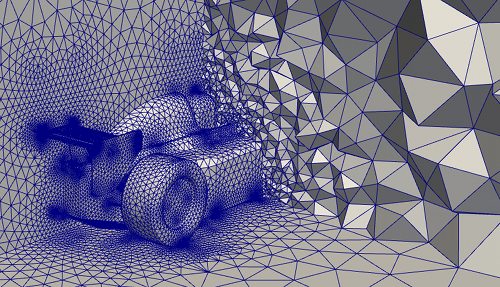
A discretization using tetrahedras

Meshing is governed by:

math shape function: used to connect the discrete values at the nodes (typical are low order polynomials).

A linear function (blue) and a piecewise linear approximation (red)

material properties: linear, aelastic, isotropic, homogenenous mat (steel) we need modulus of elasticity (Young's modulus) and Poisson strain for the component to be modeled.

Young's modulus, also known as the modulus of elasticity, is a measure of the stiffness of an elastic material and is a quantity used to characterize materials.

Young's modulus, E, can be calculated by dividing the tensile stress by the tensile strain in the elastic (initial, linear) portion of the stress-strain curve:

Tensile stress is a force (F) exerted on the original cross-section of the object A.

Tensile strain indicates the ratio between the object's change in length (ΔL) and it's original length (L0).

Poisson's ratio measures the Poisson's effect. This is what happens when you press down hard on an eraser and you also notice that it's perpendicular sides are expanding.

Rubber, for example, is an isotropic material; homogenous (the same at every point in the material) and rotationally symmetric (looks the same after a certain amount of rotations). It's tensile modulus is usually somewhere between 0.01 and 0.1, and it's Poisson ratio of approximately 0.5. QUAD4 elements can be used to determine stiffness, while tetrahedra elements can be used to to determine stress. The actual values of strains and stresses can be computed using the material properties described above.

Finetuning the mesh

To analyze areas of high interest - such as connectors - one can subdivide the mesh and observe finer details. One approach for mesh refinement is to increase the polynomial degree of an element without subdividing it in space. Or, the element can be subdivided geometrically, and various polynomial degrees can be applied to the subelements. The number of element refinement candidates easily reaches 100 in 2D and 1000 in 3D.

The hp-method (hp-FEM) combines two refinement types: size of the element (h) and polynomial degree (p). If instead of making the size of the element (h) smaller, one increases the degree of the polynomials (p) used in the basis function, one has the p-method.

FEM in practice

1 Estimate the solution
2 Select an acceptable error { define maxError }
Loop {
3 Mesh/adapt the model
4 Solve the model { return primary variables }
5 Post-process { return secondary variables }
6 Estimate error { return currentError }
} until ( currentError < maxError )
7 Validate analysis

Primary Variables (PV) include displacement, temperature, velocity and pressure, while Secondary Variables (SV) are strains, stresses, failure criterion and error. PV are piecewise continuous polynomials. SV are discontinuous polynomials.

And now for a nifty workaround: instead of modelling the outer surface of a bearing as some form of contact restraints, it can be loaded with pressure, modelling the load as a sinusoidial distributed force. Basically, the domain of freedom and displacements are specified, but restraints are not used. This is the task of the SOLVER: to produce resulting displacements of all element nodes that can move in response to the applied loads.

LS-DYNA is entirely command line driven solver and you can carve an input file yourself in a plain text editor (ASCII) or you can use something like LS-PrePost (which is free but you need a license for LS-DYNA). LS-DYNA is typically used for changing boundary conditions (such as contact between parts that changes over time), crushing, crumpling, folding sheets of metal or in transient dynamic analysis, which is a fancy term for analysing crashes, crack propagation (such applications are supported by various contact algorithms), explosions (like underwater mines) and even bird strike simulations.

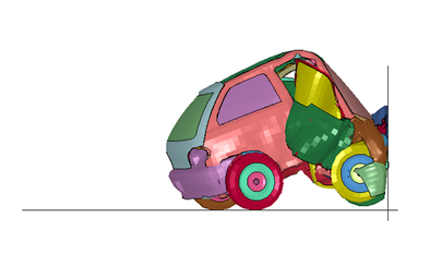
Screenshot from LS-PrePost of an LS-DYNA simulation

Just like in life, a plethora of knowledge is found on the edges and dark corners, so in order to get the model right an appropriate worst case should be considered. Such a touchstone is when a vehicle engages in cornering, breaking and bumps.

Cornering, can be simulated as a lateral load. Breaking with longitudinal loads. And the situation when the vehicle goes over a big bump can be simulated with vertical loads. Loads encompass forces, deformations and accelerations.

Non-Newtonian fluids are substances with complex molecular structure, such as blood, ketchup, custard, toothpaste, starch suspensions, paint, and shampoo. They are studied in context of stress and strain rate tensors under many different flow conditions, as opposed to Newtonian fluids which are characterized by a single coefficient: viscosity.

The Abaqus solver, which provides non-Newtonian models, can be used, for instance, to simulate the flow of blood.

A bit of history

Back in 1964, NASA realized a band of their research centers were independently developing structural analysis software. And... after putting together about one million lines of code, NASTRAN was born. It's modules (collection of subroutines aimed at solving specific tasks) are controlled by an internal language called the Direct Matrix Abstraction Program (DMAP). DMAP is a matrix oriented programming language. Below a couple of code examples, preceded by their mathematical formula:

[C] = α[A] (+,⊗,÷ ) β[B ]
ADD A,B/C/ALPHA/BETA/IOPT

[X] = ±[A] [B] ± [C]
MPYAD A,B,C/X/T/SIGNAB/SIGNC/PREC/FORM

[X] = ±[A] [B]
SOLVE A,B,SIL,USET,PARTVEC/X/SYM/SIGN/SETNAME

The most common use of DMAP is "altering" solution sequences. Take an existing solution sequence like transient response (used to compute the dynamic response of a structure over a period of time) and modify some part of its operation by inserting DMAP.

I'm sure I'm not going to surprise you by telling you that there are a bunch of software solutions for FEA. Or that there is a community of FEA DMAP programmers.

Conclusion

Finite element method is generally used to minimize error functions and produce a stable solutions for boundary value problems. This was a short introduction, focusing on it's main applications and common terminology.

It's a good start if you're working with, let's say - 3D modelling software - and came across FEM for the first time but it takes quite some time until you can get your hands dirty with actually modelling stuff using it. Head on over to Amazon Books if you want to delve deeper into this subject.

Sources:
http://www.youtube.com/watch?v=CThxYRMV8Vc&feature=list_related&playnext=1&list=SP30D4A9A59A75C20B

http://www.iue.tuwien.ac.at/phd/orio/node48.html

Shotgun Debugging

Labels

Friday, August 10, 2012

Finite Element Method for Programmers: A shotgun introduction